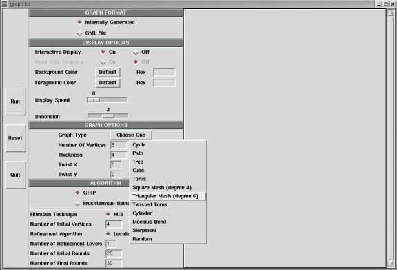
GUIDE is equipped with a flexible Tcl/Tk interface as well as a command line interface. The two interfaces are analogous to each other and hold the same capabilities, however, the graphical interface provides a more intuitive and user-friendly method for constructing desired graphs. The Tcl/Tk interface consists of 6 components: control buttons, graph format selection, display options, graph options, algorithm options and an output window. We must note that each widget is selected to provide maximum flexibility and control to the user and also that inputs are rigorously checked before being processed in order to track down user error. An overall view of the interface can be seen in Figure 1. The following sections will explain each of the components in more detail.
The GUIDE system accepts graphs in two formats. The graph format can be selected via the Graph Format panel, see Fig. 1. The first type consists of graphs generated internally by the program and stored as adjacency lists. There are twelve different graphs currently implemented, each of which requires different input parameters. The “Graph Type” field (as seen in Figure 1) allows selection of one of the following types of graphs: cycle, path, tree, cube, torus and twisted torus, meshes of degree 4 & 6, cylinder, moebius band, Sierpinski graph and a random graph. The parameters for each graph are entered in the Graph Options panel, which dynamically adjusts to the selected type of the graph. The meaning of each parameter is discussed below.
Figure 1: GUIDE Graphical User Interface.
Cycles and paths are the simplest graph types. They only require one input parameter, shown in Fig. 2 (a) & (b), which specifies the number of vertices. In a path, each vertex except for the endpoints has degree of 2. The endpoints have degree of 1. The ideal drawing of a path is a straight line that spans all the vertices. A cycle is a path where the two endpoints are connected yielding a circular drawing.
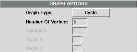
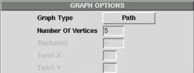
Figure 2(a) & (b): Required parameters for Cycles and Paths.
Trees require two parameters: depth and base as shown in Fig. 2(c). The depth specifies the height, or the number of levels, of the tree. The base specifies the branching factor for each subtree. For example, specifying depth = 10 and base = 2 will produce a binary tree with 10 levels and 29=512 leaf nodes. In this case the total number of vertices is 1023.
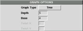
Figure 2(c): Required parameters for Trees.
The cube graph produces a hypercube of specified dimension; see Fig. 2(d). The dimension here is not synonymous with the dimension of the drawing on the screen, but specifies the structure of the hypercube. So, a 2-dimensional hypercube would produce a planar square, while a 3-dimensional hypercube will produce a regular cube. As the number of dimensions increases, the graph becomes more difficult to represent on a 2D screen and even with a 3D representation.
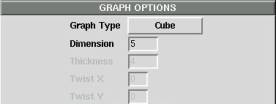
Figure 2(d): Required parameters for Cubes.
A torus has a similar structure to a cylinder with the exception that all of its vertices have a degree of 4. This means that the outer circles of the cylinder are connected to each other giving the graph a donut-like shape. As seen in Figure 2(e) the parameters for torus are also width and height. For twisted torus there are two additional parameters, twistX and twistY, seen in Fig. 2(f). They specify the degree of twisting of a regular torus in X and Y directions respectively. If we consider a torus to be a square mesh that is rolled up into a cylinder, which is then connected at its endpoints, then the twist in X direction would correspond to misaligning the edges of the mesh when it is rolled up into a cylinder. For a similar scenario, twist in the Y direction corresponds to rotating one end of the cylinder before the two ends are connected. For each twist, the value of the parameter specifies the twist magnitude in vertices.
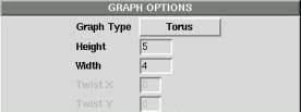
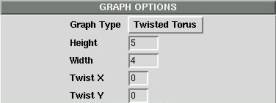
Figure 2(e) & (f): Required parameters for Tori and Twisted Tori.
There are two types of mesh graphs implemented in the GUIDE system. The square mesh, or mesh of degree 4, takes as input the height and produces a square graph of height2 vertices (see Fig. 2(g)). The triangular mesh is a mesh of degree 6, which takes the same parameter and produces a triangular graph with the given height and (height + 1)height/2 number of vertices, see Fig. 2(h).
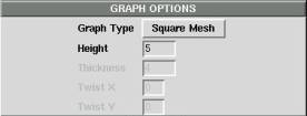
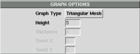
Figure 2(g) & (h): Required parameters for Square and Triangular Meshes.
A cylinder is represented by its height and width, shown in Fig. 2(i). The height to the height of the tube and the width specifies the number of vertices along one of the rings of the cylinder. The total number of vertices in the graph is w * h.
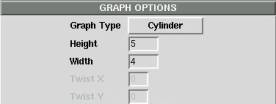
Figure 2(i): Required parameters for Cylinders.
The Moebius band draws a circular band with a single twist. As shown in Figure 2(j), the graph requires two parameters: length and thickness. The length specifies the circumference of the band in terms of vertices and the thickness denotes number of vertices that span the width of the band. The total number of vertices is defined by the product of length and thickness.
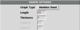
Figure 2(j): Required parameters for Moebius Bands.
The Sierpinski graph is an instance of a fractal graph. It draws a pyramid, which is recursively subdivided into 4 equilateral pyramids and has the middle one removed. For this graph, as shown in Fig. 2(k), the user needs to specify the recursion depth and dimensionality. The recursion depth specifies how many times the above recursion is to be performed. The dimensionality specifies whether the graph should be the Sierpinski triangle (0) or the Sierpinski pyramid (1).
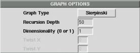
Figure 2(k): Required parameters for Sierpinski graphs.
The random graph contains randomly connected vertices. The height specifies the number of vertices in the graph. The random graph is created by first generating a base 2 tree with height number of vertices. Then vertices are randomly added to the graph up to density specified by width, see Fig. 2(l).
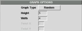
Figure 2(j): Required parameters for Random graphs.
Graphs that are read in GML (graph modeling language) format must have two properties specified by the user as seen in Figure 3. The first is the file name containing the encoding of the graph. The second is the split components flag, which indicates whether the graph should be split up into disconnected components, each of which would be processed separately by the algorithm, or the whole graph should be processed as a whole. Processing of each component separately tends to produce more appealing drawings. This flag does not affect connected graphs.
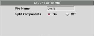
Figure 3: GML graph options.
The display options, seen in Fig. 4(a), modify the visual properties of the drawing produced by GUIDE. These are static properties that are set before the display of the drawing occurs. The drawing window has its own set of controls that will be covered in section 6. Each of the static display options is covered below.
|
|
 |
|
Figure 4: Display options panel in (a) default view and (b) color selection view. |
The Interactive Display toggle switch specifies whether the drawing should be shown progressively after each stage of processing or display should be suppressed until all stages have been completed. If interactive display is turned off, there will be a slight performance improvement due to avoiding the time cost of reading in the graph configuration and rendering it on the screen.
Each of the color selections provides three flexible interfaces for selecting a color. The color can be entered in hexadecimal format, omitting “0x”, in the entry box provided, or a common color can be selected from the drop down menu, see Fig. 4(b). If a desired color is not listed in the selection menu, choosing “Other” will pop up a custom color panel and once a selection has been made, the hexadecimal value will be stored in the display color option, as shown in Fig. 5. If no selection has been made for the color and a default value is kept, then the hex value for the default will not be displayed but will be set internally by GUIDE. The default background color is black and default foreground color is green.
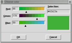
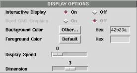
Figure 5: Custom
color selection.
The Display Speed control will only affect an interactively displayed graph. This option specifies whether a delay should occur in between drawing of different stages of the algorithm. Since the movement of vertices through each stage will occur fairly quickly, this option is useful for observing the vertex movements in slow motion.
The Dimension slider allows the user to select how many dimensions the drawing should have. Note that this will not only affect the rendering of the graph on the screen but will be used by the algorithm to produce optimal placement of vertices. The values currently supported are 2, 3 and 4. Four-dimensional drawings are projected down into 3 dimensions.
The Read GML Graphics control is only applicable to the GML graph format. Enabling this control will make sure that any graphics properties specified in the GML file are read in and used in the rendering of the graph, see Fig. 6. Such properties include direction of edges, self-loops and colors specified for vertices and edges. Note that selection of the Foreground Color in the Display Options (Fig. 4) does not override the GML color properties. It is also important to note that if the GML file does not specify a color for some vertices/edges then they will be drawn in the Foreground Color if one is selected, or the default color if no selection has been made.
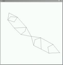
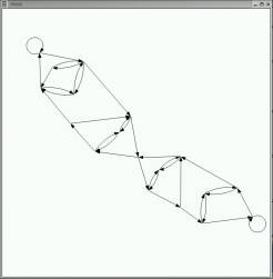
Figure 6: A graph rendered with (a) Read GML Graphics off and (b) with Read GML Graphics on.
There are two algorithms for force-directed graph drawing implemented in the GUIDE system: the GRIP algorithm and the Fruchterman-Reingold algorithm. Each algorithm has a set of options that a user can select.
There are six configurations for fine-tuning the GRIP algorithm, see Fig. 7(a). The filtration technique derives the number of processing stages in the algorithm. The default is the MIS filtration but a Random filtration is faster and tends to result in a few more levels. The number of initial vertices indicates how many vertices will be plotted in the first stage of the algorithm.
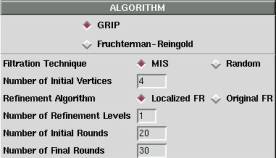
Figure 7(a): Configurable options for GRIP algorithm.
There are two refinement algorithms used in GRIP: Kamada-Kawai approximates vertex positions and Fruchterman-Reingold refines the vertex placement. The refinement algorithm option refers to the second algorithm used for a localized refinement of vertices. By default, GRIP uses the localized Fruchterman-Reingold algorithm, which only looks a few neighbors of a particular vertex to decide its final position. However, GUIDE also makes use of the original Fruchterman-Reingold algorithm, where all vertices already plotted are examined to decide the position of a vertex. The original FR algorithm is more computationally expensive but produces smoother drawings. The user can also specify the number of levels at which the refinement algorithm is applied using the number of refinement levels parameter.
The number of initial rounds parameter is the number of iterations of the refinement stages in the beginning of the program, while number of final rounds is the number of iterations of GRIP towards the end of the algorithm. The number of iterations in the intermediate stages is determined by a scheduling function that derives values between number of initial rounds and number of final rounds. Typically an increase in the number of initial rounds will place vertices more precisely in the beginning stages, and therefore the number of rounds toward the end can be significantly lowered. GRIP can provide a good drawing for most graphs with number of initial rounds between 10 and 20 and number of final rounds between 5 and 30.
The Fruchterman-Reingold algorithm utilizes three parameters, as shown in Fig. 7(b). Note that in contrast to the use of a modified version of this algorithm in GRIP, here no filtrations are constructed and the algorithm is applied to all vertices at each stage. The first two options are used for temperature calculations. The maximum possible increase/decrease in the temperature of a vertex is directly proportional to this value. The cooling/heating speed linearly decreases at each stage from the value specified by the user and levels out at 1.0. Therefore any value below 1.0 will be internally adjusted to 1.0.
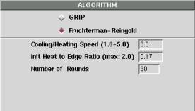
Figure 7(b): Configurable options for Fruchterman-Reingold algorithm.
The initial heat to edge ratio is a decimal value that indicates a relationship between the initial temperature of each vertex and the ideal edge length. The ideal edge length is multiplied by this value to determine the initial temperature with the reasoning that as the ideal edge length increases so must the temperature to allow farther displacement by vertices.
The number of rounds parameter the number of iterations that the Fruchterman-Reingold Algorithm will be run for. The typical value is 100 but as many as 500 rounds maybe needed to draw more complex drawings. The high range of values comes from the way the cooling function works, where it takes several dozens of rounds to move the vertices out of their random positions and closer to the optimal positions.
The graphical user interface has a set of controls consisting of 3 buttons. The Reset button will reset all values, including display options to the default values used at the start up of the interface. The Quit button will close the Tcl/Tk interface but it will not quit out of the drawing window, which has a separate set of controls that will be described below. The Run button executes the program producing a new window with the rendering of the drawing. When the drawing window is closed, the output from the program is logged in the output panel shown in Fig. 8.
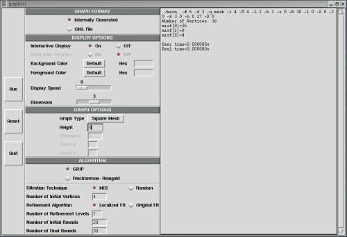
Figure 8: Output from the program, shown in the left side of the window.
The first line starting with “./main” is the actual command line interface command issued to the operating system. Each of the flags corresponds to an option chosen from the GUI. Then the number of vertices is displayed. This information is important since for graphs such as meshes, the user can’t specify the number of vertices but rather a parameter that is used to calculate the total number of vertices. The last piece of information is the size of each filtration level. It is displayed as “misf[0]=36” where 0 is the number of the level and 36 is the number of vertices at that level. The number of vertices at level 0 will always equal the total number of vertices. This information will be displayed for graphs drawn with GRIP. In addition, if the graph is run with Interactive Display off, the time that the algorithm took to run excluding the drawing process will be displayed. This can only be done with Interactive Display off because the rendering of intermediate stages of the graph will occupy CPU time and it would be difficult to distinguish between the time taken by the algorithm and the drawing process. When the program is being run, a drawing window pops up that contains the actual drawing, see Fig. 9.
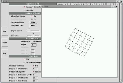
Figure 9: The drawing window on top of the GUI.
The graph is displayed using OpenGL and using capabilities of OpenGL a series of controls are provided in the drawing window. All the commands are case sensitive.
There are several commands for manipulating the viewing angle of the drawing. The drawing can be rotated in all 3 directions (x, y and z). Rotation along the x-axis can be accomplished by pressing X for clockwise rotation or x for counter-clockwise rotation. The left and right arrow keys are analogous to X and x respectively. To rotate along the z-axis, the user can use the Z key on the keyboard (or z for counter-clockwise rotation), or up and down arrows similar to above. Rotation along the y-axis can only be accomplished by pressing the Y and y keys depending on desired direction of rotation. Note that rotation is continuous and can only be stopped by pressing S (for stop). Rotation is not applicable to two-dimensional drawings.
The drawing window also has zooming capabilities. Pressing F (for forward) will zoom in on the object. Pressing B (for backward) will zoom out. Zooming is not continuous which means performing above commands will only zoom in/out by a little bit. For continuous zoom, the user must hold down the appropriate key until desired level of zoom is achieved.
The drawing interface provides the capability for moving vertices from the plotted location after all the stages of the algorithm have completed. To do so, the user must click on the vertex (or in close proximity) and while holding down the left mouse button drag the vertex to the desired location. Releasing the mouse button will move the vertex to its new location. We must note that vertex movement can be performed after zoom is performed but cannot be performed after rotation. Doing so will provide unpredictable results because displacement of a 3D vertex in 2D space provides inaccurate movement.
The S key is also functional during the intermediate stages of the drawing process. Pressing S will stop the algorithm after the current processing stage has completed and the result has been displayed. This is useful for observing properties of the graph in the middle of the algorithm. To continue the algorithm execution, the user must press the R (for resume) key. This option can be performed numerous times during the execution of the program, however, if the user wants to pause after every stage then the Display Speed should be set to 1 from the Tcl/Tk interface.
To quit the program and close the drawing window at any time during execution or after the final drawing is rendered, the Q key must be pressed. It is important that the program is always exited in this way rather than closing the window by pressing the X in the top right corner. Pressing Q ensures that all the memory used by the program is freed before the program exits.